Code
library(brms)
library(cowplot)
library(tidybayes)
library(tidyverse)
set.seed(1234)(499/500 words)
Biologging uses animal-borne sensors to remotely observe animals and their environments1. In the six decades since a biologist first attached a modified kitchen timer to a seal2, biologging has become an invaluable, multidisciplinary tool to address questions in ecology3, atmospheric science4,5, and oceanography6. As biologging data continue to grow in size and complexity (e.g., millions of new records daily in Movebank7 and novel sensors like infrasound recorders8), “big data” methods are a key direction for future developments9,10. Simultaneously, biologging data are increasingly used to inform conservation efforts across taxonomic groups11,12 and regions13. However, the envisioned impacts of aggregated biologging data on research and conservation are hindered by a lack of data standardization, discoverability, and accessibility14, which has become a growing matter of practical and ethical concern15. Currently, there is no systematic review of biologging studies, instruments used, species investigated, or open biologging datasets. Insights from such a review would support collaborative data sharing and curation efforts, and direct approaches to drive greater research and conservation impacts.
Open science practices, such as publishing data and code alongside manuscripts, improve research transparency and efficiency16,17. However, data “openness” is determined by multiple factors, and poor research data management and sharing practices are a major source of biodiversity data loss18. Fortunately, the FAIR principles19 (Table 1) provide a useful framework to facilitate open data, with FAIR data enabling groundbreaking advances in synthesis, biodiversity, and conservation science20–23 .
Numerous efforts within the biologging research community have sought to promote open data. For example, data standards14,24,25 and domain-specific data repositories (Movebank7, seabirdtracking.org, Euromammal26) facilitate the adoption of the FAIR principles (Table 1). However, the overall state of open data in biologging research remains unknown, and there are indications that most tracking data remain inaccessible27,28.
| FAIR principle | Definition | Application to biologging | Example |
|---|---|---|---|
| Findability | Data and metadata have a globally unique and persistent identifier (e.g., a digital object identifier, DOI) and are indexed in a searchable resource | Data repositories, like the Movebank Data Repository7, improve data discoverability and may assign DOIs to data (avoiding issues with broken hyperlinks, for example) | A tracking dataset deposited in the Movebank Data Repository is findable by its permanent DOI or by searching the repository |
| Accessibility | Data and metadata are retrievable by open and universal protocols, such as HTTP | Data repositories allow scientists to retrieve biologging data via a web browser or other open source tools | Publicly available data on Movebank may be downloaded via the website, API, or with the move2 R package29 |
| Interoperability | Data use formal and shared formats and vocabularies | Shared protocols like the Darwin Core standard30, Movebank data model31, and proposed bio-logging standardization framework14 reduce barriers to combining datasets and increase uptake within and across scientific disciplines | Location and environmental data from seal-borne biologgers harmonized to a standard netCDF format facilitated their reuse by oceanographers to study polar regions6 |
| Reusability | Data and metadata are richly described and reuse permissions are clearly defined | Data repositories and standards together capture essential context for biologging data and provide licensing options for data reuse | The Movebank Data Repository releases datasets under the CC0 license and the Movebank data model31 includes fields important for data reuse (e.g., whether the animal was relocated before release) |
We will conduct a systematic review to quantify the diversity of instruments, species, and open data practices in biologging studies published between 2007-2023. 2007 marked the creation of Movebank, the largest biologging data platform. Our review will test the following three hypotheses:
H1: Open biologging data practices are increasing over time.
H2: Open biologging data practices vary by ecosystem.
H3: Open biologging data practices are greater for spatial than aspatial (e.g., accelerometer) biologging data.
Beyond hypothesis testing, our review will provide the first biologging bibliometric database, itself a valuable form of cyberinfrastrucure for future systematic reviews and meta-analyses. We will also provide a minimum information standard (e.g. MIAPE33, MIReAD34) as a resource for authors, journal editors, and funding bodies to facilitate FAIR sharing of biologging data.
We will systematically review biologging studies of wild animals in the fields of ecology, evolutionary biology, and conservation science published between 2007-2023. We define biologging as animal-borne instruments with sensors and memory for data storage. Studies employing biotelemetry devices (defined as animal-borne instruments that emit a signal for an external receiver)1,35 will be excluded, because their analyses require data describing the configuration of the receiver network. We make an exception for satellite biotelemetry using the Argos network, because the Argos system resolves transmissions to timestamped locations, and thus provides researchers with data more similar to biologgers.
On 2023-08-21, we queried Web of Science Core Collection for papers published between 2007-2023 related to biologging with the following query:
animal AND (biologg* OR bio-logg* OR biotelemetry OR electronic tag* OR satellite track* OR GPS telemetry OR satellite telemetry OR satellite transmit* OR GPS collar* OR depth recorder* OR accelerometer OR archival tag*)
This yielded 6654 papers. We limited results to relevant Web of Science categories with 100+ papers, leaving 4799 papers. The categories we considered relevant were Ecology, Zoology, Marine Freshwater Biology, Biodiversity Conservation, Multidisciplinary Sciences, Environmental Sciences, Oceanography, Biology, Behavioral Sciences, Ornithology, Evolutionary Biology, and Fisheries. We excluded the following categories with 100+ papers because they typically involve domesticated or lab animals: Agriculture Dairy Animal Science, Veterinary Sciences, Engineering Electrical Electronic, Physiology, Food Science Technology, Engineering Biomedical, Agriculture Multidisciplinary, Computer Science Interdisciplinary Applications, Instruments Instrumentation.
Every paper will be separately reviewed by two individuals to assess its relevance to this review, record the presence or absence of a data availability statement, and categorize the study by sensor type, taxonomy, and ecosystem. In cases where the reviewers disagree, a third reviewer will assess the study to reach a consensus. Papers will be considered relevant if they satisfy the following two characteristics:
We will consider a paper to have a data availability statement (DAS) if it states how to access the data or explicitly states why the data are not available. Any of the following examples would be considered a DAS: “Data were deposited in a repository” with an accompanying DOI, “Data are available at a website” with an accompanying URL, “Data are available upon request”, or “Data withheld for the safety of the tracked animals”.
We will assign sensor types to one or more categories following Williams et al.36: location (e.g., GPS, depth), intrinsic (e.g., accelerometer, internal temperature), or environment (e.g., ambient temperature, camera). Biologgers can combine sensors from multiple categories (e.g., a GPS-accelerometer collar). We will consider all sensors that were reported in the methods.
We will resolve taxonomy to the species level using the Integrated Taxonomic Information System (www.itis.gov). Each study’s ecosystem will be classified as one or more of aquatic (i.e., freshwater), marine (i.e., saltwater), and terrestrial according to the IUCN Red List (https://www.iucnredlist.org).
It was necessary for us to begin the initial classification to properly design the protocol for the open data assessment (next section). We have completed the initial classification for ~25% of studies in our sample. No data have been collected about studies’ open data practices, so our hypotheses are not informed by preliminary data.
Following our initial classification, we will randomly sample 600 studies to assess the openness of biologging data. We will stratify our sample by year, ecosystem, and sensor type. We will attempt to sample 50 studies in each combination of the following categories:
Time period (early 2007-2015, middle 2016-2019, recent 2020-2023)
Ecosystem (marine, terrestrial)
Sensor type (spatial, aspatial)
Freshwater aquatic biologging studies will be excluded from the open data assessment. Our preliminary results from the initial classification indicate freshwater aquatic biologging studies are rare, as most tracking studies in this ecosystem use acoustic telemetry.
Studies may include both spatial (i.e., location) and aspatial (i.e., intrinsic or environmental) sensor data. Therefore, at the time of sampling, we will assign each study to either the aspatial or spatial category and limit our assessment to the corresponding sensor data. Our initial classification preliminary results indicate spatial sensors are deployed in the vast majority of studies (93%), whereas aspatial sensors are deployed less frequently (35% of studies).
For each sampled paper, we will attempt to retrieve the biologging dataset underlying the study. If data are available upon request, we will email the corresponding author to request the data and, if we do not receive a response within two weeks, we will send one follow-up email. Similarly, if we receive a summary of the biologging data, we will send one follow-up email requesting the underlying biologging data. We will record whether each dataset satisfies the following properties:
Findable ( \(f\) ). Do the data have a permanent identifier, such as a DOI? I.e., FAIR principle F119.
Accessible ( \(a\) ). Are the data retrievable via a standard communications protocol, such as HTTP? I.e., FAIR principle A119.
Reusable ( \(r\) ). Do the data contain biologging data (raw or processed), as opposed to descriptive statistics or other summaries? I.e., FAIR principle R119.
If we cannot retrieve the dataset for a study, we will consider the study to not satisfy any of the three properties listed above.
To clarify our methods for spatial versus aspatial data, consider a hypothetical GPS-accelerometer biologging study sampled in the aspatial category. The authors deposited the GPS data in the Movebank Data Repository (which issues DOIs) and the accelerometer data are available upon request. We contact the author and they provide us with a summary table of the accelerometer data, where each row is a deployment and columns are characteristics of the deployment, such as duration. They do not respond to our follow-up email requesting the underlying biologging data. Then, because this study was sampled in the aspatial category, it would be scored as \(f=0,a=0,r=0\) because (\(f\)) the accelerometer data do not have a DOI, (\(a\)) retrieving the accelerometer data required contacting the author, and (\(r\)) only summaries of the accelerometer data were made available. Had this same study been sampled in the spatial category, we would have scored it as \(f=1,a=1,r=1\) because (\(f\)) the spatial data have a DOI, (\(a\)) the data were retrievable via HTTP, and (\(r\)) the GPS sensor data were available.
Our independent variables will be year of publication (\(t\)), ecosystem (\(e\)), and sensor type (\(s\)) [see “Initial classification”]. Our dependent variables will be findability (\(f\)), accessibility (\(a\)), and reusability (\(r\)) [see “Assessing open data”]. We will fit three Bayesian generalized linear models of the form:
\[ \begin{align} DV &\sim Bernoulli(p) \\ logit(p_i) &= \alpha + \beta_e \times e_i + \beta_s \times s_i + \beta_t \times t_i \\ \end{align} \]
Where \(DV\) is the dependent variable (\(f\), \(a\), or \(r\)). \(e\) and \(s\) encode ecosystem (0 for marine, 1 for terrestrial) and sensor type (0 for aspatial, 1 for spatial), respectively. \(t\) is the publication year minus the beginning of the study period (i.e., \(t=0\) in 2007, …, \(t=16\) in 2023).
We use the following priors:
\[ \begin{align} \alpha &\sim Normal(0, 4) \\ \beta_e &\sim Normal(0, 2) \\ \beta_s &\sim Normal(0, 2) \\ \beta_t &\sim Normal(0, 0.5) \end{align} \]
We conducted prior predictive checks of our priors. Flatter priors, such as \(Normal(0,10)\) for all coefficients, lead to unrealistic values for \(p\) (i.e., the probability density of \(p\) is concentrated almost entirely near 0 or 1).
We will use Stan37 and brms38,39 for model fitting.
We invite feedback from reviewers about statistical design. We considered more complex models, e.g., using splines for \(\beta_t\), treating year as an ordinal variable40, or allowing interactions between \(e\), \(s\), and \(t\). However, we concluded that the model presented here would answer our research questions with the greatest clarity. If the reviewers think more complex models are essential, we will modify our design accordingly.
We will test hypotheses by testing if the 95% credible interval for the posterior probability distribution of the relevant model coefficients (in all three models) is greater than 0. We will quantify effect sizes using the 95% credible interval for the posterior probability distribution of contrasts in \(p(f)\) , \(p(a)\), and \(p(r)\) across levels of the relevant category to the hypothesis. We calculate contrasts by sampling the posterior distribution of the probability of a dependent variable (e.g., \(p(f)\)) while varying the category of interest. For example, the contrast of \(p(f)\) for hypothesis H2 (open data vary by ecosystem, \(e\)), is \(p(f|e=terrestrial)-p(f|e=marine)\), marginal across \(s\) and \(t\). See section “Analysis of simulated data” to see our implementation with simulated data.
We will test hypothesis H1 using coefficient \(\beta_t\). We will quantify effect size by contrasting the dependent variable posterior probabilities for three eras: 2007-2015, 2016-2019, and 2020-2023 (see Figure 2 in section “Analysis of simulated data” below).
We will test hypothesis H2 using coefficient \(\beta_e\). To quantify effect size, we will contrast posterior probabilities for marine and terrestrial ecosystems (see Figure 3).
We will test hypothesis H3 using coefficient \(\beta_s\). To quantify effect size, we will contrast posterior probabilities for aspatial and spatial sensor data (see Figure 4).
We conducted a simulation to demonstrate how we will conduct our analysis. We simulated values for \(t\), \(e\), \(s\) (time, ecosystem, and sensor class; independent variables), and \(f\) (findability; dependent variable) according to our predictions, to demonstrate how we will perform our analysis. The full analysis will also include dependent variables \(a\) (accessibility) and \(r\) (reusability).
We set up our analysis by loading necessary packages and setting the seed.
library(brms)
library(cowplot)
library(tidybayes)
library(tidyverse)
set.seed(1234)The following code simulates our independent and dependent variables. We simulate independent variables according to our stratified sampling plan (biolog_grid). Then we choose values for our parameters \(\beta_e\) (beta_E), \(\beta_s\) (beta_S), \(\beta_t\) (beta_T), and \(\alpha\) (alpha), which we use to simulate our dependent variable, \(f\) (F). The probability of \(f\), \(p(f)\), increases over time, and \(p(f)\) is greater for spatial sensors and terrestrial ecosystems than aspatial sensors and marine ecosystems (Figure 1).
# Grid of independent variables
biolog_grid <- expand_grid(
  era = c("early", "middle", "recent"),
  E = c("marine", "terrestrial"),
  S = c("aspatial", "spatial")
) %>%
  slice(rep(seq(nrow(.)), each = 50)) %>%
  mutate(T = case_when(
    era == "early"  ~ sample(2007:2015, nrow(.), replace = TRUE),
    era == "middle" ~ sample(2016:2019, nrow(.), replace = TRUE),
    era == "recent" ~ sample(2020:2023, nrow(.), replace = TRUE)
  ))

# Parameters for simulation
# betas (E, S, T)
alpha <- -4
beta_E <- c(marine = 0, terrestrial = 0.5)
beta_S <- c(aspatial = 0, spatial = 1.5)
beta_T = 0.2

# Run simulation
inv_logit <- \(x) exp(x) / (1 + exp(x))
biolog <- biolog_grid %>%
  mutate(T2007 = T - 2007,
         logit_p = alpha + beta_E[E] + beta_S[S] + beta_T * T2007,
         p = inv_logit(logit_p),
F = rbinom(nrow(.), size = 1, prob = p))# Visualize data
e_palette <- c(marine = "navy", terrestrial = "goldenrod")
biolog_text <- filter(biolog, T == 2023) %>%
distinct(E, S, p) %>%
mutate(label = str_to_title(paste(E, S, sep = "\n")))
ggplot(biolog, aes(T, p, color = E)) +
geom_jitter(aes(y = F, shape = S),
width = 0.25, height = 0.05,
alpha = 0.5) +
geom_line(aes(linetype = S)) +
geom_text(aes(label = label), biolog_text,
x = 2023.1, hjust = 0) +
scale_color_manual(values = e_palette) +
scale_x_continuous(limits = c(NA, 2025),
breaks = seq(2010, 2020, by = 5)) +
labs(y = expression(p(f))) +
expand_limits(x = 2025) +
theme_classic() +
theme(legend.position = "none",
axis.title.x = element_blank())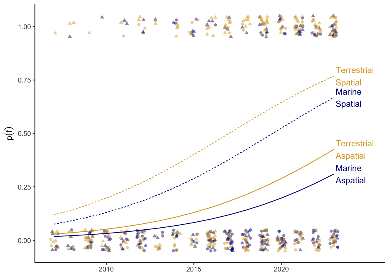
Here we specify our model, including priors, and fit it to our simulated data.
# Fit model
biolog_prior <- c(
    set_prior(prior = "normal(0, 4)", class = "Intercept"),
    set_prior(prior = "normal(0, 2)", coef = "Eterrestrial"),
    set_prior(prior = "normal(0, 2)", coef = "Sspatial"),
    set_prior(prior = "normal(0, 0.5)", coef = "T2007")
  )
biolog_mod <- brm(F ~ E + S + T2007,
                  data = biolog,
                  family = bernoulli(link = "logit"),
                  prior = biolog_prior,
                  chains = 4,
                  iter = 50000,
                  seed = 6789,
                  refresh = 0)
biolog_draws <- as_draws_df(biolog_mod)
We test our hypotheses using credible intervals of the parameter estimates and contrasts of the posterior probabilities. In our simulation, the 95% credible intervals for coefficients \(\beta_t\), \(\beta_e\), and \(\beta_s\) were greater than 0 (Figure 2A, Figure 3A, Figure 4A). The contrasts quantify the effect sizes in the simulation. Figure 2B, for example, shows the posterior distribution of the contrast of \(p(f)\) from the early to middle periods (above) and from the middle to recent periods (below). The 95% credible interval from early to middle periods was (0.073 - 0.300), indicating the probability of findability increased 7.3% - 30%.
h1_dens <- density(biolog_draws$b_T2007)
h1_dens_dat <- tibble(
  b_T2007 = h1_dens$x,
  dens = h1_dens$y,
  ci95 = between(b_T2007,
                 quantile(biolog_draws$b_T2007, 0.025),
                 quantile(biolog_draws$b_T2007, 0.975))
)

h1_contrast <- map2(
  list("early", "middle", "recent"),
  list(2007:2015, 2016:2019, 2020:2023),
  function(era, years) {
    dat <- expand_grid(
      E = c("marine", "terrestrial"),
      S = c("aspatial", "spatial"),
      T = years
    ) %>%
      mutate(T2007 = T - 2007)
    linpred_draws(biolog_mod,
                  transform = TRUE,
                  newdata = dat) %>%
      group_by(E, S, .draw) %>%
      summarize(p_F = mean(.linpred),
                .groups = "drop") %>%
      mutate(era = era)
  }
) %>%
  list_rbind() %>%
  pivot_wider(names_from = "era", values_from = "p_F") %>%
  mutate(`Early to Middle` = middle - early,
         `Middle to Recent` = recent - middle) %>%
  pivot_longer(c(`Early to Middle`, `Middle to Recent`),
               names_to = "Eras",
               values_to = "Contrast")

h1_contrast_dens <- h1_contrast %>%
  group_by(Eras) %>%
  group_map(\(rows, keys) {
    dens <- density(rows$Contrast)
    lwr <- quantile(rows$Contrast, 0.025)
    upr <- quantile(rows$Contrast, 0.975)
    cross_join(keys,
               tibble(Contrast = dens$x,
                      Density = dens$y,
                      ci_95 = between(Contrast, lwr, upr)))
  }) %>%
  list_rbind()

beta_t_ci_lwr <- quantile(biolog_draws$b_T2007, 0.025)
beta_t_ci_upr <- quantile(biolog_draws$b_T2007, 0.975)
early_middle_lwr <- with(
  h1_contrast, quantile(Contrast[Eras == "Early to Middle"], 0.025)
)
early_middle_upr <- with(
  h1_contrast, quantile(Contrast[Eras == "Early to Middle"], 0.975)
)
middle_recent_lwr <- with(
  h1_contrast, quantile(Contrast[Eras == "Middle to Recent"], 0.025)
)
middle_recent_upr <- with(
  h1_contrast, quantile(Contrast[Eras == "Middle to Recent"], 0.975)
)p_h1a <- ggplot(h1_dens_dat, aes(b_T2007, dens)) +
geom_line() +
geom_area(data = filter(h1_dens_dat, ci95), fill = "grey50") +
expand_limits(x = 0) +
labs(x = expression(beta[t]), y = "Density") +
theme_classic()
p_h1b <- ggplot(h1_contrast_dens, aes(Contrast, Density)) +
geom_line() +
geom_area(data = filter(h1_contrast_dens, ci_95), fill = "grey50") +
facet_grid(rows = vars(Eras), scales = "free_y") +
labs(x = "Contrast in p(f)") +
expand_limits(x = 0) +
theme_classic()
plot_grid(p_h1a, p_h1b, nrow = 1, labels = "AUTO")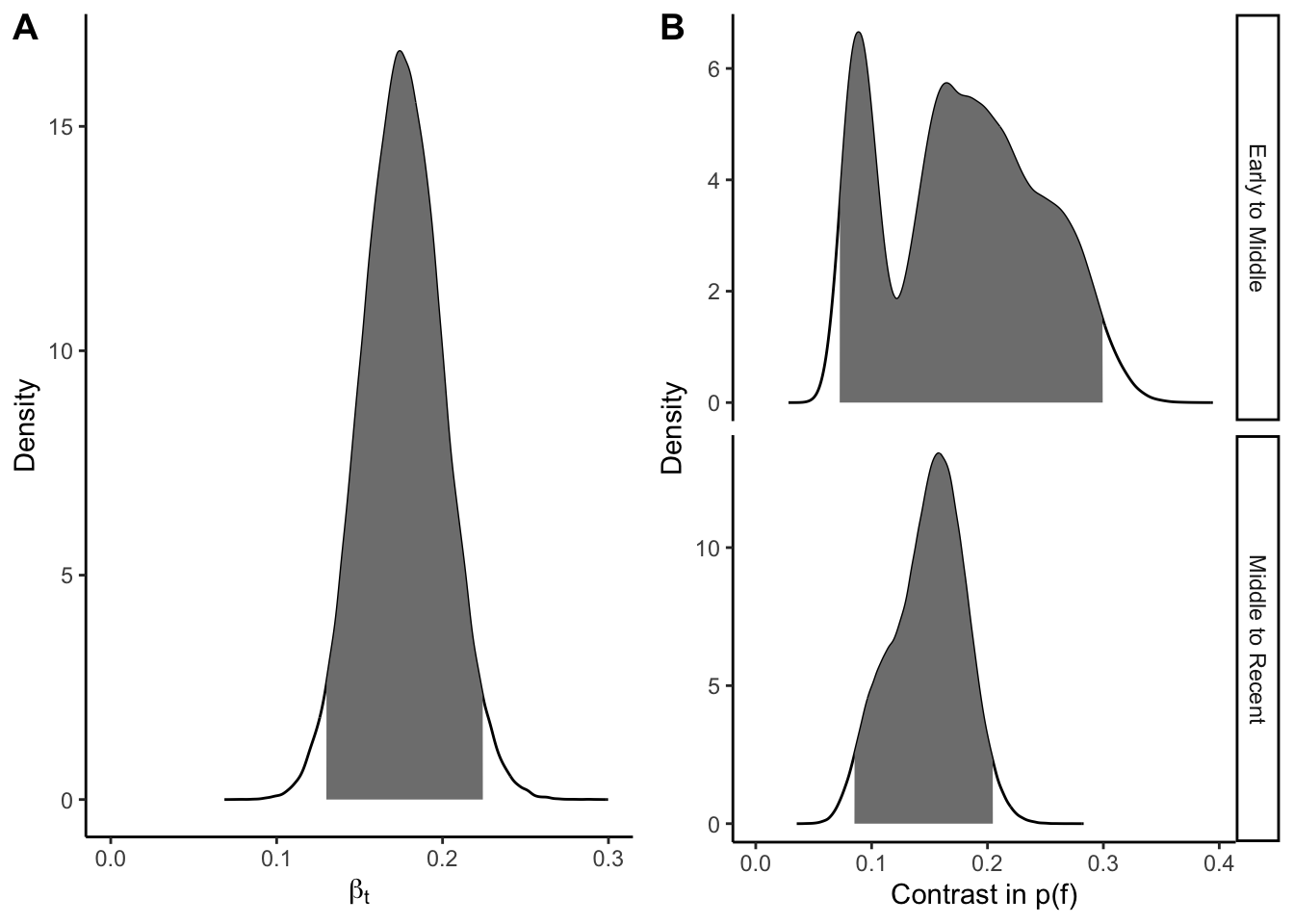
h2_dens <- density(biolog_draws$b_Eterrestrial)
h2_dens_dat <- tibble(
  b_Eterrestrial = h2_dens$x,
  dens = h2_dens$y,
  ci95 = between(b_Eterrestrial,
                 quantile(biolog_draws$b_Eterrestrial, 0.025),
                 quantile(biolog_draws$b_Eterrestrial, 0.975))
)

h2_contrast <- map(
  c("marine", "terrestrial"),
  function(e) {
    dat <- expand_grid(
      E = e,
      S = c("aspatial", "spatial"),
      T = 2007:2023
    ) %>%
      mutate(T2007 = T - 2007)
    linpred_draws(biolog_mod,
                  transform = TRUE,
                  newdata = dat)
  }
) %>%
  list_rbind() %>%
  pivot_wider(names_from = "E", values_from = ".linpred") %>%
  mutate(Contrast = terrestrial - marine)

dens <- density(h2_contrast$Contrast)
h2_contrast_dens <- tibble(
  Contrast = dens$x,
  Density = dens$y,
  ci_95 = between(Contrast,
                  quantile(h2_contrast$Contrast, 0.025),
                  quantile(h2_contrast$Contrast, 0.975))
)

beta_e_ci_lwr <- quantile(biolog_draws$b_Eterrestrial, 0.025)
beta_e_ci_upr <- quantile(biolog_draws$b_Eterrestrial, 0.975)
e_contrast_lwr <- quantile(h2_contrast$Contrast, 0.025)
e_contrast_upr <- quantile(h2_contrast$Contrast, 0.975)p_h2a <- ggplot(h2_dens_dat, aes(b_Eterrestrial, dens)) +
geom_line() +
geom_area(data = filter(h2_dens_dat, ci95), fill = "grey50") +
expand_limits(x = 0) +
labs(x = expression(beta[e]), y = "Density") +
theme_classic()
p_h2b <- ggplot(h2_contrast_dens, aes(Contrast, Density)) +
geom_line() +
geom_area(data = filter(h2_contrast_dens, ci_95), fill = "grey50") +
expand_limits(x = 0) +
labs(x = "Contrast of p(f) [terrestrial - marine]") +
theme_classic()
plot_grid(p_h2a, p_h2b, nrow = 1, labels = "AUTO")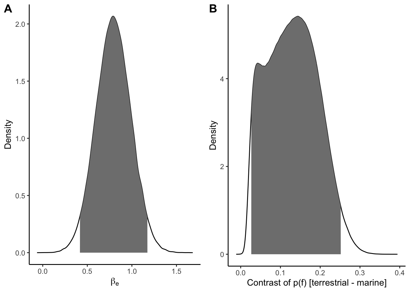
h3_dens <- density(biolog_draws$b_Sspatial)
h3_dens_dat <- tibble(
  b_Sspatial = h3_dens$x,
  dens = h3_dens$y,
  ci95 = between(b_Sspatial,
                 quantile(biolog_draws$b_Sspatial, 0.025),
                 quantile(biolog_draws$b_Sspatial, 0.975))
)

h3_contrast <- map(
  c("aspatial", "spatial"),
  function(s) {
    dat <- expand_grid(
      E = c("marine", "terrestrial"),
      S = s,
      T = 2007:2023
    ) %>%
      mutate(T2007 = T - 2007)
    linpred_draws(biolog_mod,
                  transform = TRUE,
                  newdata = dat)
  }
) %>%
  list_rbind() %>%
  pivot_wider(names_from = "S", values_from = ".linpred") %>%
  mutate(Contrast = spatial - aspatial)

dens <- density(h3_contrast$Contrast)
h3_contrast_dens <- tibble(
  Contrast = dens$x,
  Density = dens$y,
  ci_95 = between(Contrast,
                  quantile(h3_contrast$Contrast, 0.025),
                  quantile(h3_contrast$Contrast, 0.975))
)

beta_s_ci_lwr <- quantile(biolog_draws$b_Sspatial, 0.025)
beta_s_ci_upr <- quantile(biolog_draws$b_Sspatial, 0.975)
s_contrast_lwr <- quantile(h3_contrast$Contrast, 0.025)
s_contrast_upr <- quantile(h3_contrast$Contrast, 0.975)p_h3a <- ggplot(h3_dens_dat, aes(b_Sspatial, dens)) +
geom_line() +
geom_area(data = filter(h3_dens_dat, ci95), fill = "grey50") +
expand_limits(x = 0) +
labs(x = expression(beta[s]), y = "Density") +
theme_classic()
p_h3b <- ggplot(h3_contrast_dens, aes(Contrast, Density)) +
geom_line() +
geom_area(data = filter(h3_contrast_dens, ci_95), fill = "grey50") +
expand_limits(x = 0) +
labs(x = "Contrast of p(f) [spatial - aspatial]") +
theme_classic()
plot_grid(p_h3a, p_h3b, nrow = 1, labels = "AUTO")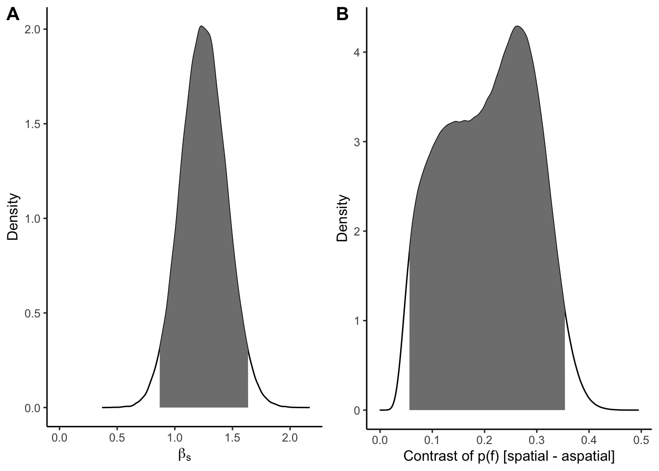
Table 1: Description of the FAIR principles and their application to biologging data (see Table 1 above).
Table 2: Results of our hypothesis tests for the three dependent variables. 95% credible intervals for posterior probability distributions of our model coefficients and contrasts. This table summarizes Figure 2, Figure 3, and Figure 4 from the section “Analysis of simulated data”, as well as results for the other two dependent variables.
Figure 1: Results of the initial classification. A Sankey diagram showing the frequencies of instrumented species by number of studies, with aggregations at higher taxa. B Frequencies of location, intrinsic, and environmental sensors used in studies. C Prevalence of data availability statements over time. D Cumulative biologging studies published over time in the ten journals with the most published biologging studies.
Figure 2: Results of the open data assessment. Mean and standard error of dependent variables (\(f\) findability, \(a\) accessibility, \(b\) reusability) aggregated over: A sensor type (aspatial or spatial), B ecosystem (marine or terrestrial), and C time (year of publication).
Supplemental figures 1-3: Posterior probability distributions of model coefficients and contrasts. Each supplemental figure will show the full posterior probability distributions for three hypotheses and one dependent variable. I.e. supplemental figure 1 would combine Figure 2, Figure 3, and Figure 4 from the section “Analysis of simulated data” above. Supplemental figures 2 and 3 would be similar, showing the results for the other dependent variables accessibility ( \(a\) ) and reproducibility ( \(r\) ).