Data collection progress

Code

library(tidyverse)

── Attaching packages ─────────────────────────────────────── tidyverse 1.3.1 ──

✔ ggplot2 3.4.2     ✔ purrr   1.0.1
✔ tibble  3.2.1     ✔ dplyr   1.1.2
✔ tidyr   1.3.0     ✔ stringr 1.5.0
✔ readr   2.1.4     ✔ forcats 1.0.0

── Conflicts ────────────────────────────────────────── tidyverse_conflicts() ──
✖ dplyr::filter() masks stats::filter()
✖ dplyr::lag()    masks stats::lag()

Code

# Get the most recent set of reviews
reviews <- dir(here::here("outputs", "reviews"), 
                      "reviews.*rds", 
                      full.names = TRUE) %>%
  sort(decreasing = TRUE) %>%
  first() %>%
  readRDS()

# And most recent studies-by-taxonomy
study_taxa <- readRDS(here::here("outputs", "taxa", "study_taxa.rds"))

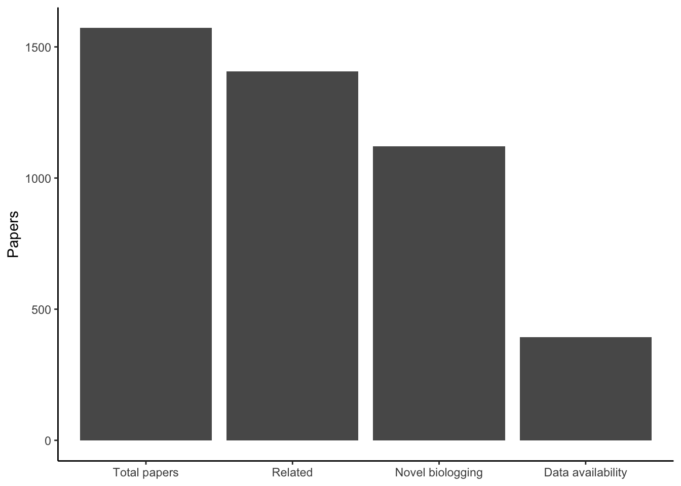
How many papers have we scored?

Code

scored_papers <- reviews %>% 
  mutate(across(everything(), \(x) ifelse(x == "NA", NA, x))) %>% 
  filter(reviewed)

nrow(scored_papers)

[1] 1572

Breakdown of papers by relatedness, novel biologging, and data availability statement.

Code

scored_papers %>% 
  summarize(
    `Total papers` = n(),
    `Related` = sum(manuscript_type != "U", na.rm = TRUE),
    `Novel biologging` = sum(novel_biologging == "Y",
                             na.rm = TRUE),
    `Data availability` = sum(biologging_availability == "Y",
                              na.rm = TRUE)) %>% 
  pivot_longer(everything()) %>% 
  mutate(name = fct_reorder(name, value, .fun = \(x) -x)) %>% 
  ggplot(aes(name, value)) +
  geom_col() +
  labs(y = "Papers") +
  theme_classic() +
  theme(axis.title.x = element_blank())

Figure 1: ?(caption)

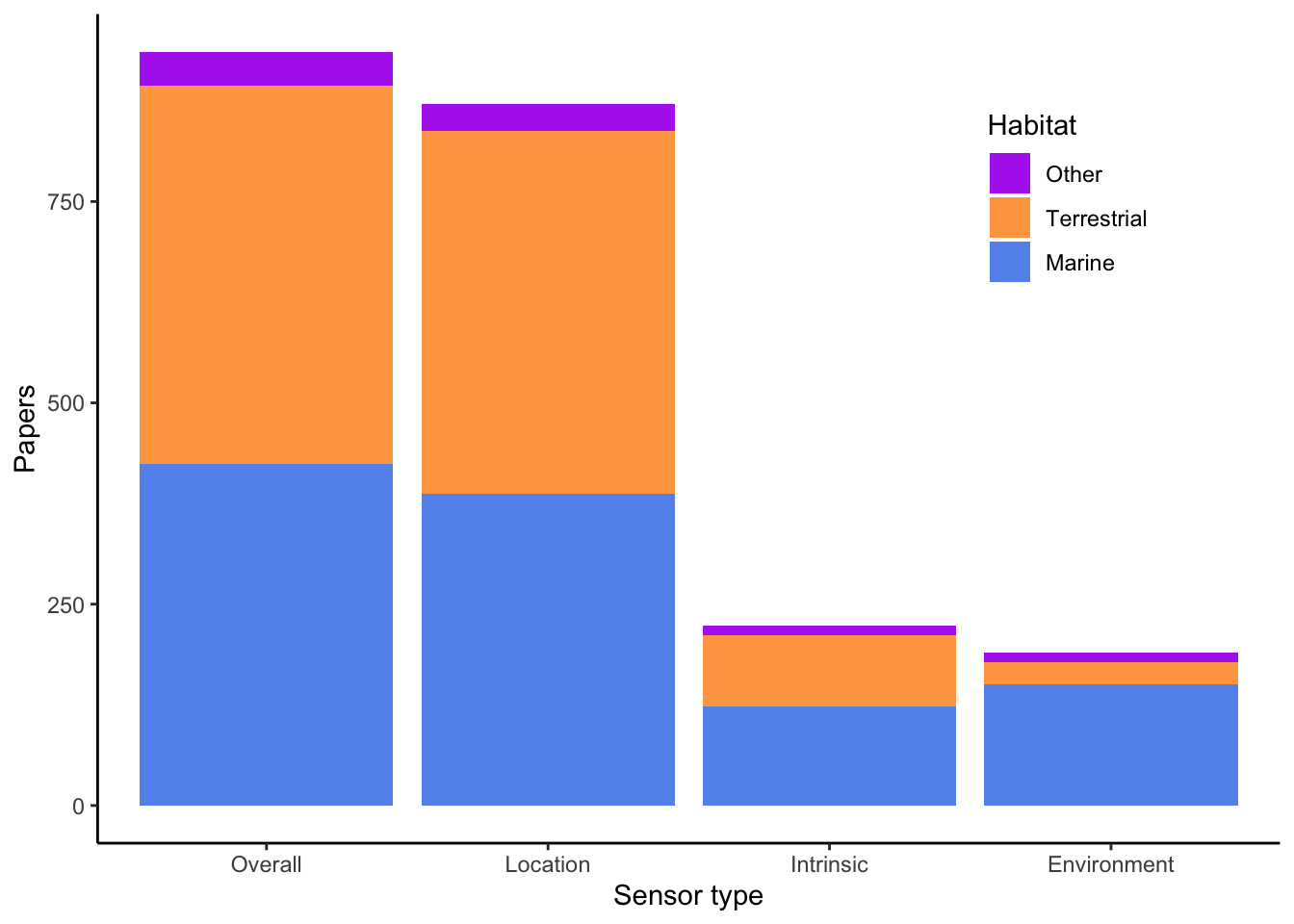
Breakdown of biologging data by sensor type. Limited to animals in the wild (no domestic or captive).

Code

novel_biolog <- scored_papers %>% 
  filter(manuscript_type != "U",
         novel_biologging == "Y",
         str_detect(biologging_context, "W"),
         !is.na(novel_biologging)) 

novel_biolog %>% 
  mutate(Habitat = case_when(
    substr(habitat, 1, 1) == "M" ~ "Marine",
    substr(habitat, 1, 1) == "T" ~ "Terrestrial",
    TRUE ~ "Other"
  )) %>% 
  group_by(Habitat) %>% 
  summarize(
    Overall = n(),
    Location = sum(str_detect(device_cat, "L"),
                   na.rm = TRUE),
    Intrinsic = sum(str_detect(device_cat, "I"), 
                    na.rm = TRUE),
    Environment = sum(str_detect(device_cat, "E"), 
                      na.rm = TRUE)) %>% 
  pivot_longer(-Habitat, 
               names_to = "Sensor type", 
               values_to = "Papers") %>% 
  mutate(
    `Sensor type` = fct_reorder(`Sensor type`, 
                                Papers, 
                                .fun = \(x) -sum(x)),
    Habitat = fct_reorder(Habitat, Papers, .fun = sum)
  ) %>% 
  ggplot(aes(`Sensor type`, Papers, fill = Habitat)) +
  geom_col() +
  scale_fill_manual(values = c(Terrestrial = "tan1",
                               Marine = "cornflowerblue",
                               Other = "darkorchid2")) +
  theme_classic() +
  theme(legend.position = c(0.9, 0.9),
        legend.justification = c(1, 1))

Figure 2: ?(caption)

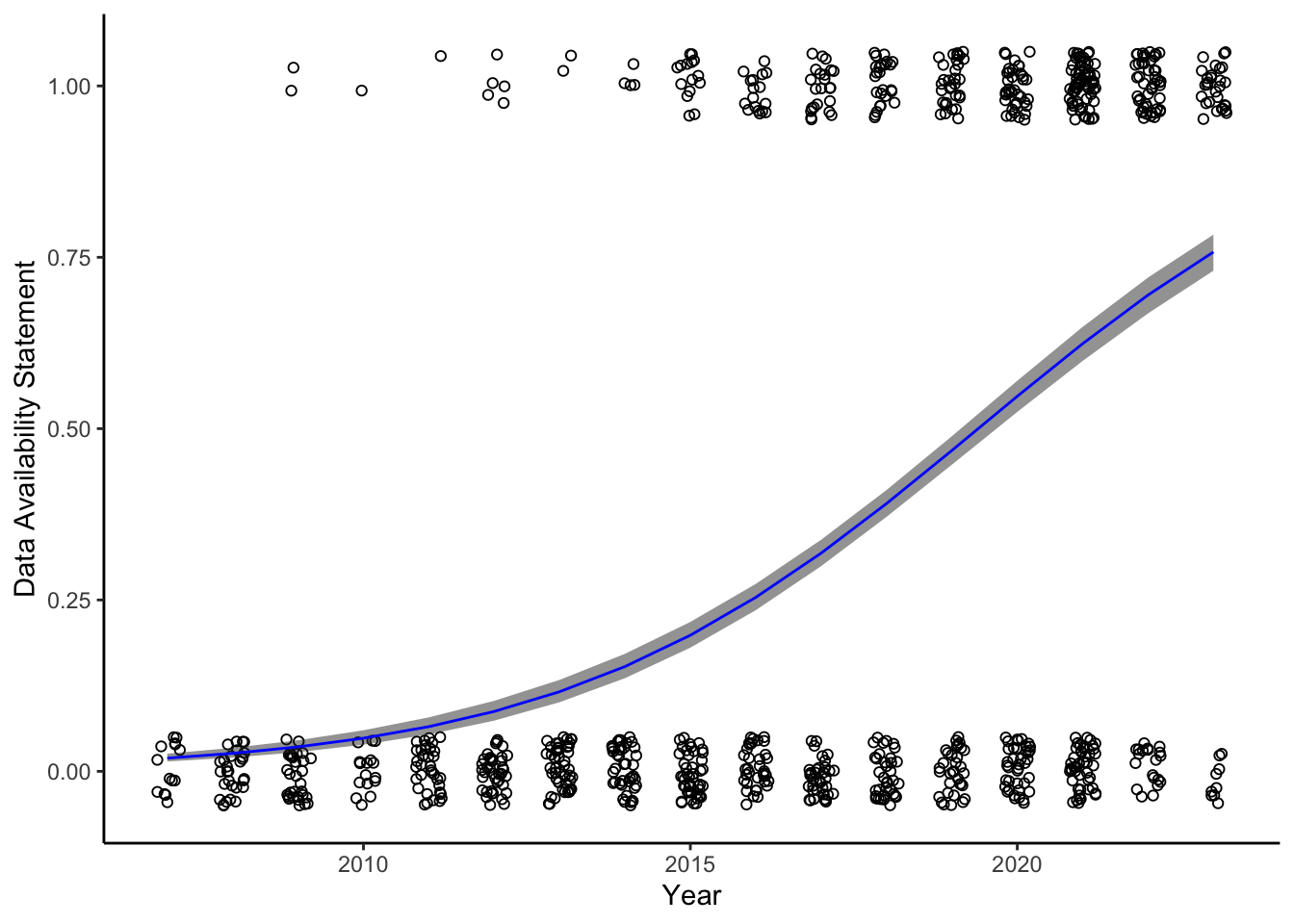
Data availability statements over time.

Code

data_avail <- novel_biolog %>% 
  drop_na(biologging_availability) %>% 
  mutate(
    biologging_availability = ifelse(biologging_availability == "Y",
                                     1, 0),
    year = as.numeric(year),
    year2007 = year - 2007
  )

data_avail_mod <- glm(biologging_availability ~ year2007,
                      family = "binomial",
                      data = data_avail)
data_avail_grid <- tibble(year2007 = 0:16)
data_avail_pred <- predict(data_avail_mod,
                           newdata = data_avail_grid,
                           se.fit = TRUE)
invlogit <- binomial()$linkinv
data_avail_pred_df <- data_avail_grid %>% 
  mutate(eta = data_avail_pred$fit,
         eta_lwr = data_avail_pred$fit - data_avail_pred$se.fit,
         eta_upr = data_avail_pred$fit + data_avail_pred$se.fit,
         biologging_availability = invlogit(eta),
         biologging_availability_lwr = invlogit(eta_lwr),
         biologging_availability_upr = invlogit(eta_upr),
         year = year2007 + 2007)

ggplot(data_avail, aes(year, biologging_availability)) +
  geom_point(shape = 21, 
             position = position_jitter(width = 0.2, height = 0.05)) +
  geom_ribbon(aes(x = year,
                  ymin = biologging_availability_lwr,
                  ymax = biologging_availability_upr),
              data_avail_pred_df,
              alpha = 0.5) +
  geom_line(data = data_avail_pred_df,
            color = "blue") +
  labs(x = "Year", y = "Data Availability Statement") +
  theme_classic()

Figure 3: ?(caption)

Taxonomic coverage of biologging.

Code

library(networkD3)
study_taxa_categorized <- study_taxa %>% 
  mutate(group1 = ifelse(phylum == "Chordata", "Vertebrate", "Invertebrate"),
         group2 = case_when(
           class == "Aves" ~ "Birds",
           class == "Mammalia" ~ "Mammals",
           class %in% c("Chondrichthyes", "Chondrostei", "Teleostei") ~ "Fish",
           group1 == "Vertebrate" ~ "Other vertebrates",
           TRUE ~ phylum
         ),
         group3 = case_when(
           order == "Carnivora" ~ "Carnivores",
           order %in% c("Artiodactyla", "Perissodactyla") ~ "Ungulates",
           order == "Cetacea" ~ "Cetaceans",
           class == "Mammalia" ~ "Other mammals",
           order %in% c("Charadriiformes", "Sphenisciformes", "Procellariiformes", "Suliformes", "Pelecaniformes") ~ "Seabirds",
           order %in% c("Anseriformes", "Galliformes") ~ "Fowl",
           order %in% c("Accipitriformes", "Falconiformes", "Strigiformes") ~ "Raptors",
           class == "Aves" ~ "Other birds",
           TRUE ~ NA
         ))

category_sizes <- study_taxa_categorized %>% 
  pivot_longer(group1:group3, names_to = "group", values_to = "category") %>% 
  count(category) %>% 
  drop_na()
links <- rbind(
  select(study_taxa_categorized, source = group1, target = group2),
  select(study_taxa_categorized, source = group2, target = group3)
) %>% 
  drop_na(source, target) %>% 
  count(source, target) %>% 
  left_join(select(category_sizes, source = category, source_n = n), 
            by = "source") %>% 
  left_join(select(category_sizes, target = category, target_n = n), 
            by = "target") %>%
  mutate(source = str_glue("{source} ({source_n})"),
         target = str_glue("{target} ({target_n})"))
  
nodes <- tibble(
  name = unique(c(links$source, links$target))
)

links$IDsource <- match(links$source, nodes$name) - 1
links$IDtarget <- match(links$target, nodes$name) - 1

sankeyNetwork(Links = as.data.frame(links), 
              Nodes = as.data.frame(nodes),
              Source = "IDsource", Target = "IDtarget",
              Value = "n", NodeID = "name", 
              sinksRight = FALSE, fontSize = 14, fontFamily = "Helvetica")